Lecture 1: Overview, Tokenization

1.1 Overview

Overview: 5 assignments at github about

• basics: implement tokenizers, optimizers, transformers, loss functions
• systems: implement profiling harness, checkpointing, flashattention kernels, parallelism methods
• scaling: experiment about scaling laws
• data: implement data extraction, filtering and deduplication
• alignment: implement DPO and GRPO

1.2 Tokenizer

Tokenizer works for:

• encoding unicode strings into tokens (indices)
• decoding tokens into unicode strings

Anderj Karpathy’s lecture

Unicode and Word Tokenizer have a too large vocalbulary size (150K) and too many rarely-used tokens though they have good compression rate ( original byte length / token length ).

Byte Tokenizer has a small vocalbulary size (256) but compression rate is 1.

Byte Pair Encoding (BPE) Tokenizer starts from the byte vocalbulary (256), and then iterates on the byte sequence by finding the most frequent pair, adding it into the vocalbulary and translating the past token sequence into the new one. The number of iteration should be carefully chosen.

Tokenizer may be abandoned from LMs by learning from bytes e2e, but for now transformers still work on chunks in some form.

Lecture 2: Resource Accounting

2.1 Data types

float32: single precision, 8 bits of exponent, 4 bytes.

float16: half precision, 5 bits of exponent, 2 bytes. Poor dynamic range, underflow frequently.

bfloat16: 8 bits of exponent, 2 bytes. More dynamic range.

Mix precision training: bf16 for parameters, activations and gradients, fp32 for optimizer states. Pytorch has an automatic mixed precision (AMP) library, tries to cast things to bf16 when it’s safe.

fp8 (2022): E4M3 has 4 bits of exponent while E5M2 has 5 bits of exponent.

nvfp4 (2025): 4 bits with a separate scale factor per block.

Low bits often happen in inferencing with quantization.

2.2 Einops

einops: a library for manipulating tensors where dimensions are named.

• einsum notifies the dimension changing by naming when matrix multiplications and transposing happen.
• reduce notifies the dimension changing by naming when summing happens.
• rearrange notifyes the dimension changing by naming when matrix rearranging (mostly about spliting and grouping a specific dimension) happens.

2.3 FLOP

FLOP: a floating-point operation like addition or multiplication. FLOPs is the number of FLOP done while FLOP/s or FLOPS is the number of FLOP per second (used to measuring hardwares). Sometimes hardwares have performances with sparsity like 50%, which means the real performance should be weighted by sparsity.

FLOPs for a MatMul is 2 * B * D * K when x (B x D) @ w (D x K) and there are a multiplication and a addition for all triples (Fused Multiply-Add like a * b + c). MatMuls often need quite more FLOPs than elementwise operation (O(B D) for a B x D matrix) and addition of two matrices (B * D for two B x D matrices), hence we usually account MatMuls only. 2 * B * D * K can also be seen as 2 * #tokens * parameters where B is the number of data points and (D K) is the number of parameters. FLOPs for a backward pass is twice as FLOPs for a borward pass like 4 * B * D * D.

From FLOPS to actual wall-clock time:

• time it with cuda synchronization and divide FLOPS with real time.
• or use the specification sheet for promised FLOP/s (depends on hardware and data type).

Model FLOPs utilization (MFU): actual FLOP/s / promised FLOP/s. MFU $\geq$ 0.5 is quite good (even higher when MatMuls dominate).

2.4 Arithmetic Intensity

Accelerator intensity: FLOP/s / bytes_per_sec

Arithmetic intensity: FLOPS / bytes

Bottelneck:

• Memory-bound: communication time (bytes input and output / bytes_per_sec) > computation time (flops / FLOP/s). Also arithmetic intensity < accelerator intensity.
• Compute-bound: communication time < computation time, also arithmetic intensity accelerator intensity.

Training Transformers involves big matrix multiplications (compute-bound when batch size is large enough) while inference involves matrix-vector product (memory-bound).

2.5 Memory

• Parameters: 2 * D * D * L (2 bytes for bf16)
• Activations: 2 * B * D * L (2 bytes for bf16)
• Gradients: 2 * Parameters (4 bytes for fp32)
• Optimizer States: 4 * Parameters (4 bytes for fp32 of stability). 4 bytes/parameter for AdaGrad to store second moments, and Adam requires 8 bytes/parameters for storing first and second moments.

Compute FLOPS (one step for training) = forward pass + backward pass = Parameters + Gradients = 6 * D * D * L.

Memory Optimizaitons:

• Gradient accumulation (micro batch): compute gradients on micro batches and accumulate them. Every batch_size / micro_batch_size steps, update the parameters and zero out the gradients.
• Activation checkpointing (recompute): keep only activations at subset of layers in a forward pass, and recompute the missing activations from the last checkpoint in the backward pass.
  • Store all layers: activation memory is O(L) and no recomputation.
  • Store no activations: activation memory is O(1) and compute is O($L^2$) as it recomputes from the start for each layer.
  • Store every $\sqrt(L)$ layers: activation memory is O($\sqrt(L)$) and O($\sqrt(L)$) recomputation as it recomputes from a layer with distance $\sqrt(L)$ at most.

Lecture 3: Architectures

There are common senses (from afterhand proofs) and disagreements.

3.1 Pre-vs-post norm (common sense)

Pre-norm: $x_{l+1}=x_l+FFN(LayerNorm(x_l))$. No affection on the main residual signal path hence improving stability and larger LRs for large networks though it’s originally stated to be used to remove warmup. Gradient spikes are also reduced. Almost all modern LMs use pre-norm except BERT.

Post-norm: $x_{l+1}=LayerNorm(x_l+FFN(x_l))$.

Non-residual post-norm: $x_{l+1}=x_l+LayerNorm(FFN(x_l))$. Also no offensive to the main residual signal path. Used by Grok, Gemma 2 and Olmo 2 while the former 2 combine it with pre-norm (double norm).

3.2 LayerNorm vs RMSNorm (common sense)

RMSNorm computes faster than LayerNorm and has roughly the same performance. It gets rid of small operations of GPU to increase arithmetic intensity in runtime (different from FLOPS), also reduces data movement.

Details can be seen in another blog.

Bias terms are dropped in modern implementations of Transformer for simplicity in memory and optimization stability.

3.3 Activations

Gated activations: equiping GLUs with gates such as

$$FF_{ReGLU}(x)=(max(0,xW_1) \otimes xV)W_2$$

GeGLU used Gemma and SwiGLU used by LLaMa. Gating is usually helpful at performance according to experiments of Sheezer at 2020 and so on.

Gated FFN has 3 matrices comparing to 2 matrices of FFN. To ensure the #parameters be the same, the dimension of FFN ($d_{ff}$) is 2/3 of the original.

3.4 Serial vs Parallel layers

According to PaLM:

• Serial layers: $x_{l+1}=x_l+MLP(LayerNorm(x+Attention(LayerNorm(x))))$. Most
• Parallel layers: $x_{l+1}=x_l+MLP(LayerNorm(x))+Attention(LayerNorm(x))$. Originally in GPT-J (a variation of GPT-3) for faster training but tends to perform worse than serial ones possibly due to less depth.

3.5 Position embeddings

Transformers need position embeddings because the SDPA itself doesn’t account for positions.

Sine embeddings (original transformer), absolute embeddings (GPT-1/2/3), relative embeddings (Google T5).

Rotary position embeddings (RoPE, used by most LMs now): rotate every 2 dimensions of a vector at difference frequencies according to the dimension. It promises the embeddings to be invariant in absolute positions and the inner products to be invariant in relative position.

A lot of these embeddings can work, such as propotinal RoPE of Gemma 4.

Details shown in blog.

3.6 Hyperparameters

Feedforward - model dimension ratio: for ReGLU, what’s out dimension of $W_1$ or the internal hidden dimension of FFN ($d_{ff}$), and out dimension of $W_2$ or the main stream dimension ($d_{model}$)?

$$d_{ff}=4d_{model}$$

except for:

• GLU variants: scale down by 2/3 hence $d_{ff}=\frac{8}{3}d_{model}$. Mistral-7B uses 3.5 instead.
• T5: $d_{ff}=65536,\;d_{model}=1024$ since they state accelerators are most efficient for matrix multiplications in FFN. But in T5 v1.1 it’s 2.5 and Gemma 2 it’s 8x while in Gemma 3/4 it’s 4x.

Head_dim * num_heads - model-dim radio: since multi-head self-attention is released,

$$d_{head} * num_heads = d_{model}$$

Aspect ratios: how deep and how wide should a model be? We can fix $d_model / n_layer$ to a constant which most models use around 100. Deeper models are much more harder to parallelize.

Vocabulary sizes: monolingual models are about 30-50k vocab, while multilingual / production systems are about 100-250k vocab.

3.7 Regularization

Dropout loses favor these years because people have a lot more data than parameters and there are rare overfittings, but weight decay stays.

[Andriushchenko et al 2023] finds weight decay doesn’t control overfitting, but interacts with learning rates where larger LR decay results in minimum training loss.

3.8 Stability

Stability issues usually arise from a few suspects:

Softmaxes: exponents and divisions. Used before output and in attention.

• Ouput softmax stability - the ‘z loss’:
  penalizes $\log^2(Z)$ instead of $\log(Z)$ to encourage $Z(x)$ to be close to 0, where $\log(P(x))=\log(\frac{e^{U_r(x)}}{Z(x)})=U_r(x)-\log(Z(x))$ and [Devlin 2014] makes $L=\log(P(x))-\alpha\log^2(Z(x))$. Also seen in DCLM, OLMo 2/3.

• Attention softmax stability - the ‘QK norm’:
  adds layernorms on QK before they multiply with each other. Originally from vision and multimodel models, and seen in most LMs nowadays such as Gemma 2/4, Qwen 3.

We can sense from here that throwing a norm to where is instable is usually helpful.

Logit soft-capping: soft-capping logits to some maximum value via tanh. It’s a very strong stabilization introduced in Gemma but must work with QK-norm or other operations to save performance.

3.9 Attention for Serving

In prefill, arithmetic operations are $bnd^2$ and memory accesses are $bnd+bhn^2+d^2$, where b is batch size, n is sequence length and d is model dimension.

In serving, we store KVs in memory for efficiency (KV Cache), which makes the arithmetic intensity small. Arithmetic operations are the same, but memory accesses are raised to $bn^2d+nd^2$.

MQA: multiple queries use just one dimension for keys and values. KV head_num is set to 1.

GQA: multiple queries use fewer dimension for keys and values. KV head_num is set to larger than 1 less than Q head_num. Fast with minor loss in performance. Adopted by most LMs.

MLA: from DeepSeek V3, which express Q, K, V as functions of a lower-dim ‘latent’ activation for less memory. Also they have MTP to have small, lightweight models that predict multiple steps (actually 1) ahead.

Sparse / sliding window attention (SWA): does attention in local range. Current standard trick is to interleave ‘full’ and ‘local’ attention. There is NoPE (no positional embedding but causal bitmasks) for long-range info and RoPE + SWA for short-range info. Qwen 3.5/Qwen 3 Next uses gated delta rule instead of sparse attention. DeepSeek V3.2 introduces DSA for cheap attention by training a indexer to find most influential tokens needed. This area is still popular for exploring long context capability.

Lecture 4: Attention Alternatives

4.1 Linear Attention

For the long context, full attention is slow for its quadratic complexity. Linear attention and its descents are made for linear complexity.

A bunch of Gated Recurrent Units with LSTM-like state-space formulations. Linear attention emerges with the idea that $(Q^TK)V=Q^T(KV)$, Mamba2 extends it with more gate weights. They are of linear time complexity but easily forget because of weighted summation of previous inputs.

DeepSeek Attention (DSA, actually a sparse attention) builds a brute-force indexer to extract a subset of tokens really meaningful for the full attention. The Q, Ks can be projected into a lower rank for efficiency as they aren’t requiring high accuracy.

$$W=\sum\nolimits_i w_i ReLU(q_i^T k_i)$$

4.2 Mixture of Experts (MoE)

Again, the method details in another blog.

MoEs are rule of thumb but not easy to train because of routing and the overwhelming number of parameters. Different experts are good at different jobs but no human-readable semantics in their division of labor.

RL and linear fitting are heuristic but aren’t hard to train or too expensive, while top-k and hash are straightforward.

For top-k routing, DeekSeek (V1-2), Grok and Qwen use input passing gates as weights to mix FFN outputs, while Mixtral, DBRX, DeepSeek V3 use Softmax and inner products as weights.

DeepSeek and OlMoE have careful ablations for MoE and shared MoE.

Training MoE:

Main issue: expert starvation.

• RL to learn routers (Clark et al 2020)
• Stochastic approximations or noise perturbation (Shazeer 2017, Fedus 2022)
• Heuristic balancing losses or load balancing losses like per-expert, per-device (to balance device compute because experts are in seperate devices), auxiliary / auxiliary-free (Fedus 2022, DeepSeek V1/2/3). OlMoE has good ablations showing load balancing losses are meaningful to balance token loads. They are like a reinforcement on experts to even their effort and reward.

MoEs can be computed by block sparse matrix multiplication which piece computation into big diagonal-like matrices that are nice to GPUs. MegaBlocks is one of modern libraries support more smart MMs.

LatentMoE: project input tensor to low-rank to alleviate communication overhead of experts.

Upcycling: initialize a MoE with a pre-trained dense model such as instantiate the experts with one of its MLPs (MiniCPM, Qwen MoE, less seen nowadays).

Issues with MoEs:

• Bumping: silently drop tokens when the queue of one expert is too long in early years. Now fixed.
• Instability: Softmax in MoE routing is dangerous, for which we use float32 just for the expert router and auxiliary z-loss for reducing spikes.
• Fine-tuning: overfit on smaller fine-tuning data. So we either fine-tune non MoE FFNs and attention, or more data.

Lecture 5: GPUs, TPUs

5.1 GPU

Compute: streaming multiprocessors (SMs) are the controllers that can do different jobs in the same time, which itself are a bundle of compute chips. In A100, there are 128 SMs. Threads are the smallest unit of compute and parallelism, and all threads execute the same instructions but with different inputs (SIMT). Warps are the smallest scheduling unit that have 32 consecutively numbered threads, and they are the smallest implementation of SIMT. Blocks are groups of threads, and each of them runs on a SM with its own shared memory (so a block is uniquely belong to a SM, but a SM isn’t neccessarily controlling only one block). Tensor Cores are introduced since V100 for faster matmul.

Memory: most GPUs have a memory hierachy of L1 cache, L2 cache and global memory. L1 cache resides in compute chips, L2 cache lays under them and global memory connects to them. Shared memory resides in SMs and is different from caches.

Strengths:

• easily scales up hard workload (by adding more SMs)
• easier to program due to SIMT
• threads are ‘lightweight’ and can be stopped and started

Scaling: compute scaling is faster than memory scaling and communication scaling (like PCLe 5.0 and MVLink 4.0).

5.2 TPU

More optimized for the ML workload with dedicated scalar units, vector units (VPU) and matrix multiply units (MXU), hence it has lightweight control and fast matmul.

High bandwidth memory (HBM) of slow memory and Smem of fast memory.

There are corresponding concepts between GPUs and TPUs. SM in GPU is tensor core in TPU, and Tensor Core in GPU is MXU in TPU. The biggest difference lies in their number of units, where TPU has only 2 tensor cores and 8 MXUs because they are much larger than those in GPU.

Details in jax scaling book.

Trends: StepFun 3 has separate attentions and mlps on different chips in decode because the former are memory-bound for KV-cache while the latter are compute-bound for large matmuls. They called it Attention-FFN disaggregation. Nowadays, model providers (like AWS) have tried to separate prefill and decode on different chips. There has been a trend that developing chips dedicated to prefill or decode. However, communication efficiency or bandwidth is always a major obstacle.

5.3 Make ML Workloads Fast

Due to the roofline model, high enough operational intensity (flops/bytes) touches the roof of throughput (gflops). So we need to minimize memory operations while maximizing computation.

Control divergence: because of SIMT, if statements split threads of a warp by instructions hence part of them have to stay idle during the other part working.

Memory Trick 1 Low precision computation:

• Arithmetic intensity doubles for a float16 number operation as to a float32.
• Fast matmuls with precision downcasting.

  FP16 / BF16 is suitable for matmuls and most pointwise operations, FP32 / FP16 (more precision) for adding small values to large sums and reduction operations (e.g. sum, softmax, norm), FP32 / BF16 (more range) for pointwise operations where $|f(x)| \gg |x|$ (e.g. exp, log, pow) and loss functions (gradients).
  FP8 has very small range and precision, so it has to use a scaling factor for a matrix of data. NVIDIA Blackwell use multiple scaling factors MXFP8, which form scaling factors also a matrix, and make its transpose so hard that it store its transpose at its instantiation.

Memory Trick 2 Fusion:

Fuse multiple operations in one process of GPU, which reduces memory movement and enlarge flops/bytes. Pytorch Compile can automatically process simple operation fusions, and the complicated ones need dedicated CUDA kernel code.

Memory Trick 3 Recomputation:

Reduce memory movement by saving a certain part of the activations and recompute the remaining during backward pass. Trade compute for memory efficiency.

Memory Trick 4 Coalescing:

The registers always reads data by a burst or row (e.g. 32, 64, 128 bytes) not single bytes, so consecutive data reads often faster than those non-consecutive. Arrange your data consecutively helps in memory efficiency.

Memory Trick 5 Tiling:

Tiling means you read and process data not one by one, but tile by tile, which reduce memory operations from N times to N/T times. Multiple threads can share the data tile transferred once into shared memory. Tiling is affected by tile sizes, shared memory sizes, coalesced memory access, and divisibility of the matrix dim (impacting on utilization), hence memory alignment and a good tile size choice are crucial. Pytorch mode ‘max-autotune’ can automatically sweep and search for the optimal settings for GEMM.

A mystery of matrix

• Tiling is most efficient with a size of 16 or 32 because of coalescing limit of cache lines.
• Periodic behavior exists in efficiency when the matrix size goes up because the tile account amplifies in a burst other than step by step (e.g. $\frac{1792}{256}\times\frac{1792}{128}=7\times 14=98$, $\lceil\frac{1793}{256}\rceil\times\lceil\frac{1793}{128}\rceil=8\times 15=120$. If using A100 of 108 SMs, this means there are most of SMs stay idle because the workload isn’t balanced.)

5.4 FlashAttention

Details can be found in another blog. The most significant change is the incremental softmax.

Lecture 6: Kernels, Triton, XLA

6.1 CUDA Overview

Occupancy: num_warps / max_warps. This is usually low because one SM has limited number of registers (e.g. B200 has 65536 registers and 64 warps at most per SM). For example on B200, if threads_per_block=128, registers_per_thread = 160, then number_registers_per_block=20480 and num_blocks=3, so num_warps=12 and the occupancy is 18.75%. We can have a thread doing multiple operations so this is not too bad.

Bank confilts (shared memory): shared memory is divided into 32 banks, each 4 bytes (word / FP32) wide and 32 banks work in a interleaving manner. Each cycle, each bank can only be accessed by one thread and multiple threads would be serialized. This is unavoidable like in matmuls. The worst case is a warp accessing accessing distinct addresses but mapping to the same bank (e.g. $bank(addr)=\lfloor \frac{addr}{4}\rfloor \mod 32, hence $bank(32t)=bank[0]$). One solution is padding the rows making it 32 X 33, then $33t \mod 32 = t$, the other solution is referencing physical columns as $c \xor r$, which results in the same mapping as padding.

Memory coalescing (HBM): when 32 threads in a warp access HBM ,memory accesses combined into transactions of 128 bytes (cache lines), so the best case is all threads access the same cache line.

Block occupancy: make thread block account divide #SMs. Details in (A Mystery of a Matrix)[#53-Make-ML-Workloads-Fast].

6.2 Benchmarking, profiling

Benchmarking (e.g. torch.utils.benchmark) measures the wall-clock time of performing some operation, only giving us e2e time. It’s useful to compare different implementations and understand how performance scales (e.g. with dimension).

Benchmarking procedures:

1. Warmup by run the callable a few times becuase first times might be slower due to compilation, etc, and we need steadily timing.
2. Time the callable with CUDA events for accurate GPU timing without capturing CPU overhead.
3. Synchronize and Record.
4. Repeat step 2 and 3 muptiple times.

Profiling: more details in timing internal operations of multiple runs are useful for speed bottleneck detection and callable comprehension. Also need warmup first. Pytorch has torch.profiler.profile, and Nsight is more powerful.

6.3 Triton

torch.compile compiles a callable into a triton kernel that is usually slower than a builtin kernel.

Compare Triton with CUDA:

• CUDA (developed by NVIDIA) specify what each thread does, hence producing fine-grained control but more complexity for managing shared memory, etc.
• Triton (developed by OPENAI) specify what each thread block does. Generally powerful enough and only operates with HBM.

Triton operations need data to be divided into blocks (consecutive lines of data, seen as vectors). Then call a triton kernel with specifying the input and output, and finally get the output.

A block-fit-in Triton kernel works like:

Input: input_addr, output_addr (HBM)

1. Find the block id, get the addresses of this block of data from input_addr (looks like CUDA when the data you want isn't actually a block).
2. Create a mask, load the current block of data with the mask.
3. Do the calculations, intermediate variables can be created without specifying their types.
4. Store the block in output_addr with the mask.

If the data size is larger than BLOCK_SIZE, we have to break it down into multiple tiles in our Triton kernel where we actually process the data part by part with iteration.

Lecture 7: Parallellism

7.1 Building Blocks

Collective operations: conceptual primitives of distributed programming. Here Rank is a particular device/GPU, and World size is the total number of devices.

Operations:

• Broadcast: copy from rank 0 to all ranks. e.g. rank 0 loads initial checkpoint and broadcasts to all ranks.
• Scatter: scatter a tensor on rank 0 to all ranks.
• Gather: gather pieces from all ranks to rank 0 to form a tensor.
• Reduce: reduce pieces from all ranks to rank 0, applying some operation (e.g., sum, min, max).
• All-gather: perform gather to all ranks. More frequently used than gather. e.g. in tensor parallelism, gather to get full parameters for forward pass.
• Reduce-scatter: perform reduce on each dimension, scatter results. More frequently used than scatter. e.g., in backward pass, sum gradients from different data shards and distribute.
• All-reduce: reduce-scatter + all-gather. e.g., in a backward pass, sum all gradients from different data shards and replicate full parameters.
• All-to-all: each rank sends each other rank some tensor. e.g., each rank sends column 0 to rank 0, column 1 to rank 1 and so on. Frequently used in MoEs. For balanced splits, all-to-all looks like transpose.

Hardware:

• Home: PCI(e) bus (v7.0, 242GB/s), Ethernet (~200MB/s).
• Data center: 8 GPUs per node, NVLink to an NVSwitch (B200 NVLink 5.0, 1.8TB/s, 4x slower than HBM 8TB/s). 256 nodes per pod, Infiniband (~0.05TB/s). N pods per cluster, Ethernet.

Remote Direct Memory Access (RDMA): supported by NVLink and Infiniband, allows one GPU to directly read/write another GPU’s memory without involving the CPU (while Ethernet has to pass through the CPU by copying data to kernel socket buffer, building TCP packets and copying NIC ring buffer).

GB200/GB300 NVL72: 8 GPUs per tray, 9 trays per rack -> 72 GPUs in one NVLink domain.

*RDMA over Converged Ethernet (RoCE): similar to ROMA but cheaper/weaker than Infiniband, used by Meta.

NVIDIA Collective Communication Library (NCCL): translates collective operations into low-level packets that are sent between GPUs. It detects topology of hardware, optimizes the paths between GPUs, and launches GPU kernels to send/receive data.

PyTorch distributed library: torch.distributed provides clean interface for collective operations, supports multiple backends for different hardware (CPU: gloo, GPU: nccl) and higher-level algorithms.

e.g. collective_operations_main

import torch.distributed as dist

spawn(collective_operations_main, world_size=4)

def collective_operations_main(rank: int, world_size: int):
    setup(rank, world_size)

    # waits for all processes to reach here
    dist.barrier()
    data = tensor([0., 1, 2, 3], device=cuda_if_available(rank)) + rank # input and output
    dist.all_reduce(tensor=data, op=dist.ReduceOp.SUM, async_op=False) # modifies tensor
    dist.barrier()

    cleanup()


def setup(rank: int, world_size: int)
    # Specify where master lives (rank 0), used to coordinate (actual data goes through NCCL)
    os.environ["MASTER_ADDR"] = "localhost"
    os.environ["MASTER_PORT"] = "15623"
    
    if torch.cuda.is_available():
        dist.init_process_group("nccl", rank=rank, world_size=world_size)
    else:
        dist.init_process_group("gloo", rank=rank, world_size=world_size)

def cleanup():
    torch.distributed.destroy_process_group()

Benchmarking: effective bandwidth = full_sent_bytes / total_duration, sent_bytes ~ 2 (send + receive) * data_size_bytes * steps (world_size - 1 in all-reduce), total_duration = world_size * duration, independent of world size and topology.

7.2 Distributed Training

Data parallelism: split the data. Each rank loads its own piece of data, forward and backward pass, all-reduce the gradients to average all gradients.

Tensor parallelism: split parameter tensors by dimension. Each rank loads its own piece of parameter, forward and backward pass, all-gather the activations and concatenate them to get the full activation. Usually used in a node of 8 GPUs.

Pipeline parallelism: split the model by layers. Each rank gets its own piece of layers, processes micro batches and sends its output to the next rank. The pipeline bubbles can be overlapped by sending and receiving the batch processed (communication) and processing the next batch (computation).

Sequence parallelism (RingAttention): split the token sequence. Usually used for longer context and less activation memory.

Expert parallelism: store experts in different GPUs, router use All-to-all to send tokens towards their chosen experts.

Jax/TPUs: define the model, the sharding strategy and the Jax compiler handles the rest.

Parallelism details in another blog.

Lecture 8: Train with Parallelism

8.1 Multi-machine scaling.

• TPU networking: toroidal mesh, high-speed with the neighbor, good for tensor parallelism.
• GPU networking: all to all up to 256 GPUs like a tree where we have a superpod and 32 nodes, good for expert parallelism.
• TPU8i networking: closer to tree-style topologies.
• TPU8t scale-out networking: ‘virgo’ with switched networks.
• Huawei Ascend 910C Cloud Matrix: chip capacity much weaker, but combined with more chips and higher HBM capacity and bandwidth, more power cost.

8.2 Standard LLM parallelization primitives

Details in my blog. Here we only talk about their cost.

Data parallelism:

• Naive DDP: 1 all-reduce for avgeraging and copying gradients, communication cost is the gradients (2 * #param).
• ZeRO stage 1: 1 reduce-scatter to send gradients and 1 all-gather to collect full params (2 * #param).
• ZeRO stage 2: multiple reduce to send a layer’s gradients to its worker (adds up to be 1 reduce-scatter of #param) and 1 all-gather to collect full params, 2 * #param in total. Incrementally use and free the layers to reduce overheads.
• ZeRO stage 3 (FSDP): multiple all-gather to collect a layer’s params for a forward pass, multiple all-gather to collect a layer’s params for a backward pass, multiple reduce to send a layer’s gradients to its worker. 2 all-gather (#param) and 1 reduce-scatter (#param), 3 #param in total. Actually it immediately frees params and grads, and overlaps communication and computation making all-gather*s happen all at once while forward happens.

Issues:

• batch size > #machine has an unhealthy scaling.
• ZeRO stage 3 does not reduce activation memory.

Model parallelism: splits up params but communicates activations compared to ZeRO stage 3. Includes PP, TP, SP, EP.

Pipeline parallelism:

• Naive: use micro-batches to reduce bubbles, but bubbles still exist when a forward pass ends and a backward pass begins. The ratio of bubble time to useful compute is (#stages - 1) / #micro (hence batch size should be large when #stages scales). Good because only communicate activations in a point-to-point way.
• 1F1B: nearly zeros out the bubbles by computing a foward pass of micro batch B and next a backward pass of micro batch A to be feed the neighbors. However, the optimizer step is always to be synchronized so bubbles exist.

Tensor parallelism:

• Forward pass: 1 all-reduce after the computation.
• Backward pass: 1 all-reduce before the computation.
• Split: columnwise in QKV, rowwise in attention output, replicated in norms, routers, etc.
• Pros: no bubble, no complexity and no batch size requirements.
• Cons: much larger communication. Hence only used within a node (8 at most for GPUs, more for TPUs).

Activation memory is dynamic and huge. TP splits out only the matrix multiplies in attention and MLP but not LayerNorm, Dropout and inputs to attention and MLP.

Sequence parallelism: splits up LayerNorm and Dropout layers along the sequence axis by reduce-scattering TP’s output to LayerNorm and Dropout layers and all-gathering their output for next TP’s input. TP + SP fully divides the memory of all tensors.

Expert parallelism: better than TP in router dispatching, MoE and combining, but complicated in implementation (e.g., DeepEP and HybridEP). EP dispatchs experts to different DP ranks. High TP in attention, low TP in MLP and EP in MoE MLP.

Context parallelism: extends the maximum context length with Ring Attention.

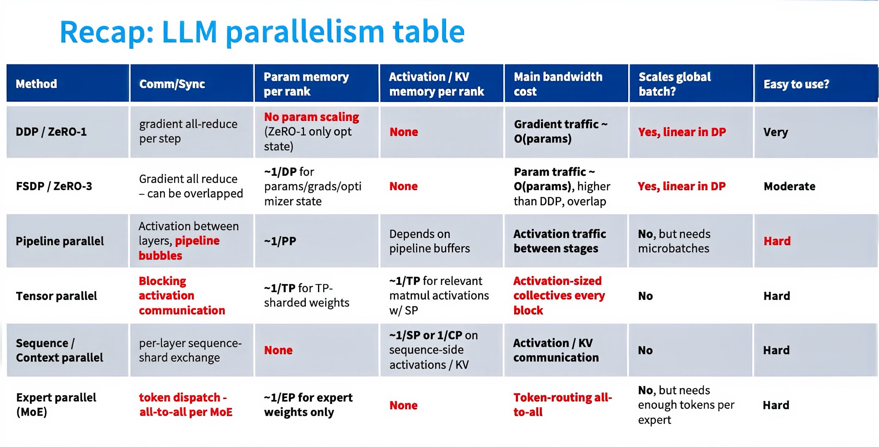
Scaling strategies from Narayanan 2021:

1. TP fisrt up to 8, then caps out at 8.
2. PP goes up to make the model fit.
3. DP gradually decreases with scale, with the largest model having DP=6 (initially 32).

Lecture 9: Scaling Laws

9.1 Early works (data scaling)

Training a classifier on a huge training set is expensive, so we want to detect the tendency in a small size.

1. Learning Curves: Asymptotic Values and Rate of Convergence, Cortes et al 1993.
2. Log-linear scaling with data, Banko and Brill et al 2001.
3. Power law relation between data and downstream performance, Kolachina et al 2012.
4. Predictable scaling on MT, LM, Speech and hypothesized scaling shape (slow, power-law, inrreducible), Hestness et al 2017.

9.2 Neural scaling behaviors

The paper, Scaling Laws for Neural Language Models, Kaplan+ et al 2020, OpenAI, found the power-scaling relationship between test losses and compute, dataset size and parameters.

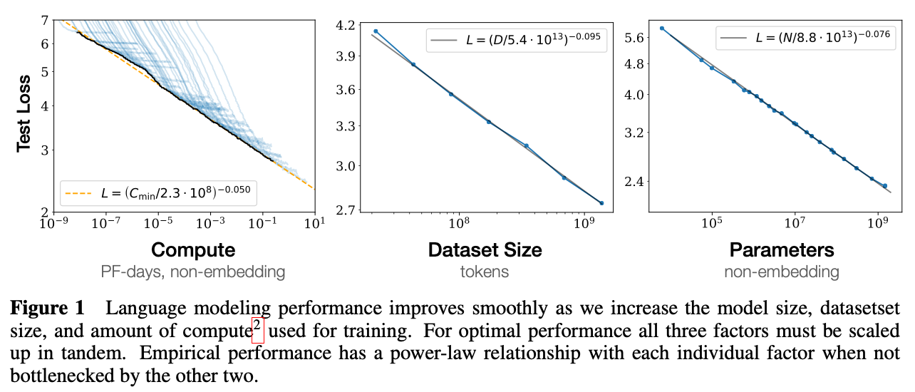
Data scaling laws: simple formula that maps data size to error. Expected to be monotonic, logistic-like curves.

Example:
Here are n numbers ($x_1, x_2, …, x_n \sim \mathcal{N}(\mu, \sigma^2)$). Estimate the mean as $\hat{\mu}=\frac{\sum\nolimits_i x_i}$.
Error $E[(\hat{\mu}-\mu)^2]=\frac{\sigma^2}{n}, hence $\log(E)=-\log n +2\log\sigma$.
Any polynomial rate $\frac{1}{n^\alpha}$ is a scaling law.

Related questions:

1. Data mixing law: hard to select data mixture via scaling (Ye et al 2024), and the practice is to just take the best small dataset (Magnusson et al 2025).
2. Data repetition: loss goes down and up with increasing epoches. The slope doesn’t change with scaling but the intercept (Kim et al 2025).
3. Data selection: data filtering should be less aggresive if the compute is growing (Goyal et al 2024).

Model scaling:

1. Architecture: train a bunch of small models to figure out the trends;
   • LSTM has worse slope and intercept with scaling (Kaplan+ et al 2021);
   • Cross-architecture scaling (Tay et al 2022).
2. Optimizer choise: Adam has a similar slope with SGD but a better intercept than it (in recurrent highway nets, Hestness+ et al 2017).
3. Depth / Width:
   • 1 layer much worse than 2;
   • Adding more layers has less and less return in slope;
   • Different size of models has a similar optimal aspect ratio (width / depth);
   • Exclude embedding then we’ll see the scaling (Kaplan+ et al 2020);
   • In MoEs, larger sparsity makes the optimal total parameters larger, while the optimal active parameters smaller (Abnar et al 2025).
4. Batch size: there is a critical batch size, smaller than which we have a perfect scaling, while larger than which it’s an ineffective scaling. It seems that smaller the target loss you want, larger the critical batch size we need. We can compute by
   1. Pick a target loss and train to get the steps needed (S) and examples needed (E);
   2. Sweep over batches;
   3. The curve follows roughly $\frac{S}{S_{min}-1}=(\frac{E}{E_{min}-1)^{-1};
   4. $B_{crit}=\frac{E_{min}}{S_{min}}$ (McCandlish et al 2018, OpenAI).
5. Learning rates: wider the model is, smaller the learning rate, usually as a function of 1 / width (Yang et al 2022);

Caution

Scaling is preditable on pre-training perplexity, but no as good in downstream metrics (Tay et al 2023).

Key takeaways: because of the belief on scaling laws, we must do a few smaller experiments to predict the possible gap between hyperparameters, and choose the optimal based on the scaling law prediction, such as optimizer choice, model depth and architecture choice, etc.

Model / Dataset Size: here are joint data-model scaling laws, from Rosenfeld+ et al 2020, $Error=n^{-\alpha}+m^{-\beta}+C$ and from Kaplan+ et al 2020, $Error=[m^{-\alpha}+n^{-1}]^\beta$.

Kaplan claims: $N_{opt}=C^{0.73}, D_{opt}=C^{0.27}$, so tokens per param decreases with C.

However, Chinchilla (Hoffman et al 2022) argues the fit is quite off and the multiplier should be about 20. It has 3 methods with different assumptions.

1. Minimum over runs: the envelope of minimal loss per FLOP over the union of all training curves is a power law. A bit tricky because the definition of a envelope is ambiguous;
2. IsoFLOPS: pick a range of FLOP budgets, vary the total parameter count and take the minimum over these convex shapes. These minima form a power law. May be the most practical and straight-forward one;
3. Joint fits: run a bunch of models on the size-data grid, choose dots with the same FLOPs and use least squares to fit a joint scaling law. A bit tricky because the curve fitting is of multiple choices. Slightly flawed in Hoffman’s paper hence its metrics are different from method 1 and 2.

Chinchilla aims to tell you what gives the best model for fixed training compute, but we should ‘over’ train since most of the compute in a real deployment is inference. For example, Mistral 7B trains 110 tokens / param, Llama 3 70B trains 215 tokens / param, etc.

Porian et al 2024 found Kaplan removed the last layer param from the parameter count, warmup was too high at small compute budgets and decay might be not critical if batch / LR was properlly tuned.

Lecture 10: Inference

10.1 Inference workload

Metrics:

1. Time-to-first-token (TTFT): how long user waits before any generation happens (for interactive applications);
2. Latency (seconds/token): how fast tokens appear for one query (for interactive applications);
3. Throughput (tokens/second): how fast tokens appear for many queries (for batch processing).

Two stages of inference:

1. Prefill: given a prompt, encode into vectors (parallelizable like in training because of causal masks);
2. Generation: generate new response tokens (sequential because future tokens isn’t predictable).

Arithmetic intensity:

MLP (bf16)

1. Read $X$ (B x T x D) from HBM: bytes += 2*B*T*D;
2. Read $W_{up}$ (D x F), $W_{gate}$ (D x F), $W_{down}$ (F x D) from HBM: bytes += 3*2*D*F;
3. Compute $U=X @ W_{up}$: flops += 2*B*T*D*F;
4. Write $U$ (B x T x F) to HBM: bytes += 2*B*T*F;
5. Compute $G=X @ W_{gate}$: flops += 2*B*T*D*F;
6. Write $G$ (B x T x F) to HBM: bytes += 2*B*T*F;
7. Compute $Y=GeLU(G) @ U @ W_{down}$: flops += 2*B*T*D*F;
8. Write $Y$ (B x T x D) to HBM: bytes += 2*B*T*D;
   intensity = flops / bytes = B*T (assume B*T much smaller than D and F).

Attention (bf16, here S is number of previous tokens, T is number of next tokens)

1. Read $Q$ (B x T x D), $K$ (B x S x D), $V$ (B x S x D) from HBM: bytes += 2*B*T*D + 2*B*S*D + 2*B*S*D;
2. Compute $A=Q @ K$: flops += 2*B*S*T*D;
3. Compute $Y=softmax(A) @ V$: flops += 2*B*S*T*D;
4. Write $Y$ (B x T x D) to HBM: bytes += 2*B*T*D;
   intensity = flops / bytes = S*T / (S+T).

1. Prefill MLP intensity: B x S (prompt length); Prefill attention intensity: S/2; Compute-bound.
2. Generation MLP intensity: B; generation attention intensity: T/(T+1) < 1(impossible to improve); Memory-bound.

Latency and Throughput: when batch size (B) grows, latency gets worse (in linear) but throughput grows (worse than linear, $\frac{100x}{x+10}$-like).

10.2 Lossy shorcuts

Reduce KV cache size:

1. MQA, GQA, MLA decrease both memory and latency but enlarge throughput;
2. Cross layer attention (CLA) computes KV cache for only a subset of layers and reuse them in other layers;
3. Sliding window attention (SWA) only store KV cache for the last fixed number of tokens, however hurting the accuracy. Hence we interleave SWA layers and global attention layers;
4. Linear attention and its variants (Mamba, etc) compress full KV cache into a fixed-length latent vector to keep memory low. They are more RNN than attention.
5. Diffusion models: LLaDA, DFlash, etc.

e.g. DeepSeek-V4:

• Compressed sparse attention (CSA): compresses every m tokens into 1;
• DeepSeek sparse attention (DSA): selects the top k KV compressed tokens, combines them with sliding window KV tokens;
• Heavily compressed attention (HCA): compresses even more.

Quantization: reduce the precision to save memory for high throughput.

1. Quantization-aware training (QAT): during training, quantize-and-dequantize during forward pass to simulate quantization errors (like in rate-aware training of 3DGS). Cons are the requirement of expensive large-scale training;
2. Post-training quantization (PTQ): run on sample data to determine scale and zero point for each layer or tensor. GPTQ (Frantar et al 2022) use Hessian information to update non-quantized weights for quantization error;
3. Activation-aware quantization (AWQ): based on observation that some activation channels are large and then weights that hit those matter more, allocate more precision to those salient weights (fp16 for the salient, int3 for the rest).

Model pruning (Muralidharan et al 2024, NVIDIA): rip out parts of an expensive model to make it cheaper, fix it up with distillation and iterate. The ripped are chosen based on activation-based importance scores (e.g, attention weights) on a small calibration dataset.

10.3 Double-checking shortcuts

Speculative sampling (leviathan et al 2022, chen et al 2023): since prefill is compute-bound and gives probabilities, use the target model to check a few tokens guessed by a small draft model.

In practice, make draft model close to target with distillation.

Medusa (Cai et al 2024) makes draft model generated multiple tokens in parallel, and EAGLE (Li+ et al 2024) makes draft model take high-level features from target model.

10.4 Handle dynamic workloads

Continuous batching: originally in a batch, request prompts are of various lengths and ends in different lengths hence padding is necessary. However in non-attention computation, we can concatenate all the sequences together.

PagedAttention: moreover, we split KV cache into pages to better sharing of KV prefixes.

Details in another blog.